Tutorial 6: Application on Slide-seq mouse Cerebellum dataset.

In this vignette, We performed PROST on the processed mouse cerebellum dataset from (Samuel G. et al. 2019) to evaluate the computational efficiency.
The original data can be downloaded from google drive.

---

1.Load PROST and its dependent packages

import numpy as np
import scanpy as sc
import os
import pandas as pd
import warnings
warnings.filterwarnings("ignore")
import matplotlib.pyplot as plt
import sys
from sklearn import metrics
import PROST
PROST.__version__


>>> ' 1.1.2 '

2.Set up the working environment and import data

# the location of R (used for the mclust clustering)
ENVpath = "your path of PROST_ENV"            # refer to 'How to use PROST' section  
os.environ['R_HOME'] = f'{ENVpath}/lib/R'
os.environ['R_USER'] = f'{ENVpath}/lib/python3.7/site-packages/rpy2'

# init
SEED = 818
PROST.setup_seed(SEED)

# Set directory (If you want to use additional data, please change the file path)
rootdir = 'datasets/Slide-seq/'

input_dir = os.path.join(rootdir)
output_dir = os.path.join(rootdir, 'results/')
if not os.path.isdir(output_dir):
    os.makedirs(output_dir)

# Read data
adata = sc.read(input_dir+"used_data.h5")

3.Plot annotation

# Plot annotation
plt.rcParams["figure.figsize"] = (4,4)
sc.pl.embedding(adata, basis="spatial", color="annotation",size = 8, show=False, title='annotation')
plt.axis('off')
plt.savefig(output_dir+"annotation.png", dpi=600, bbox_inches='tight')

4.Calculate PI

# Calculate PI
adata = PROST.prepare_for_PI(adata, percentage = 0.01, platform="Slide-seq")
adata = PROST.cal_PI(adata, platform="Slide-seq")

# Save PI
adata.write_h5ad(output_dir+"/PI_result.h5")

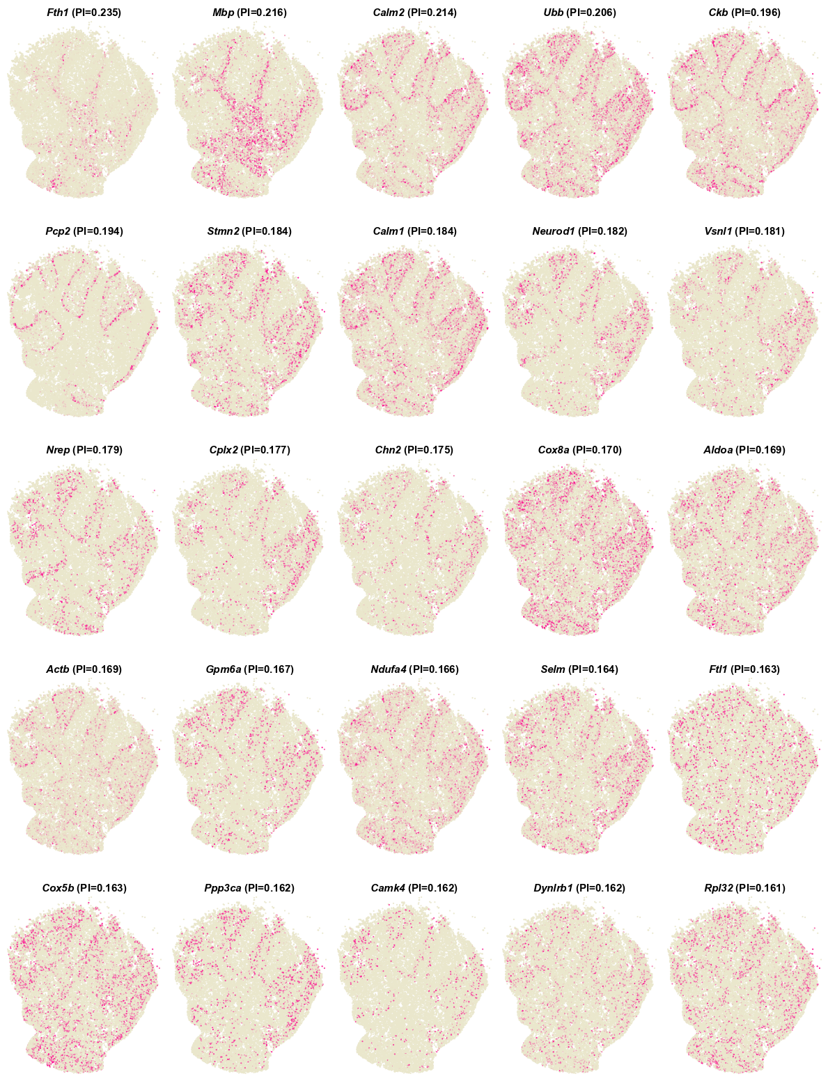
# Draw SVGs detected by PI
PROST.plot_gene(adata, platform="Slide-seq", sorted_by='PI', size = 0.3, top_n = 25, ncols_each_sheet = 5, nrows_each_sheet = 5,save_path = output_dir)
  

>>> Filtering genes ...
>>> Trying to set attribute `.var` of view, copying.
>>> Normalization to each gene:
>>> 100%|██████████████████████| 2193/2193 [00:00<00:00, 3513.47it/s]
>>> Gaussian filtering for each gene:
>>> 100%|██████████████████████| 2193/2193 [06:08<00:00,  5.96it/s]
>>> Binary segmentation for each gene:
>>> 100%|██████████████████████| 2193/2193 [00:07<00:00, 305.77it/s]
>>> Spliting subregions for each gene:
>>> 100%|██████████████████████| 2193/2193 [00:24<00:00, 88.86it/s]
>>> Computing PROST Index for each gene:
>>> 100%|██████████████████████| 2193/2193 [06:15<00:00,  5.83it/s]
>>> PROST Index calculation completed !!
>>> Drawing pictures:
>>> 100%|██████████████████████| 1/1 [00:19<00:00, 19.73s/it]
>>> Drawing completed !!

---

Clustering on original data

# Set the number of clusters
n_clusters = 8     # same as annotation

1.Expression data preprocessing

PROST.setup_seed(SEED)
# Read data
adata = sc.read(input_dir+"/used_data.h5")

sc.pp.normalize_total(adata)
sc.pp.log1p(adata)

2.Run PROST clustering

PROST.run_PNN(adata, 
        platform="slide-seq", 
        min_distance = 80,
        init="mclust",
        n_clusters = n_clusters,                   
        tol = 5e-3,
        SEED=SEED,
        max_epochs = 25)


>>> Calculating adjacency matrix ...
>>> Running PCA ...
>>> Laplacian Smoothing ...
>>> Initializing cluster centers with mclust, n_clusters known
>>> Epoch: : 27it [19:21, 43.02s/it, loss=0.1746949]             
>>> Clustering completed !!

3.Calcluate ARI

ARI = metrics.adjusted_rand_score(adata.obs["annotation"], adata.obs["clustering"])
print("pp_clustering_ARI =", ARI)


>>> pp_clustering_ARI = 0.3332276319944897

5.Save clustering result

adata.obs["clustering"].to_csv(output_dir + "/clustering.csv", header = False)
np.savetxt(output_dir + "/embedding.txt", adata.obsm["PROST"])
adata.write_h5ad(output_dir + "/PNN_result.h5")

6.Plot clustering result

adata = sc.read(output_dir + "/PNN_result.h5")
plt.rcParams["figure.figsize"] = (5,5)
sc.pl.embedding(adata, basis="spatial", color="clustering", size = 10,  show=False, title='clustering')
plt.axis('off')
plt.savefig(output_dir+"/clustering.png", dpi=600, bbox_inches='tight')

---